Tutorial 1 - Getting Started

In this first tutorial notebook we will be creating a simple KAN model and train it to perform function fitting.

from jaxkan.models.KAN import KAN

import jax
import jax.numpy as jnp

from sklearn.model_selection import train_test_split
from sklearn.metrics import mean_squared_error

from flax import nnx
import optax

import matplotlib.pyplot as plt
import numpy as np

import os
os.environ["TF_CPP_MIN_LOG_LEVEL"] = "2"

Data Generation

We begin with the generation of some mock data. Consider the function \(f(x, y) = x^2 + 2\exp(y)\). We will attempt to fit a KAN model on synthetic data generated from this function and then evaluate its performance.

def f(x,y):
    return x**2 + 2*jnp.exp(y)

def generate_data(minval=-1, maxval=1, num_samples=1000, seed=42):
    key = jax.random.PRNGKey(seed)
    x_key, y_key = jax.random.split(key)

    x1 = jax.random.uniform(x_key, shape=(num_samples,), minval=minval, maxval=maxval)
    x2 = jax.random.uniform(y_key, shape=(num_samples,), minval=minval, maxval=maxval)

    y = f(x1, x2).reshape(-1, 1)
    X = jnp.stack([x1, x2], axis=1)

    return X, y

seed = 42

X, y = generate_data(minval=-1, maxval=1, num_samples=1000, seed=seed)

Preprocessing

With the data at hand, we may perform the usual train/test splitting.

X_train, X_test, y_train, y_test = train_test_split(X, y, test_size=0.2, random_state=seed)

print("Training set size:", X_train.shape)
print("Test set size:", X_test.shape)

Training set size: (800, 2)
Test set size: (200, 2)

Note that the shapes of the objects are (batch, input_dim).

KAN Model

Selecting and initializing a jaxKAN model is straightforward. Here we focus on the most basic model, KAN, where one needs to define the following arguments, which are universal for all KAN Layer types:

• layer_dims: The dimensions for each of the network’s layers’ input/output nodes.

• layer_type: The type of KAN layer to use, which defaults to base (more details can be found in the next tutorial for other layer types).

• seed: An integer for reproducibility.

Apart from these, there is also the required_parameters argument, which is simply a dictionary with keys that correspond to additional parameters of the specific chosen layer.

We will use a Chebyshev Layer for the present example. Note that not only other layer types, but also other models can be used instead of KAN (examples can be found in subsequent tutorials).

# Initialize a KAN model
n_in = X_train.shape[1]
n_out = y_train.shape[1]
n_hidden = 6

layer_dims = [n_in, n_hidden, n_hidden, n_out]
req_params = {'D': 5, 'flavor': 'exact'}

model = KAN(layer_dims = layer_dims,
            layer_type = 'chebyshev',
            required_parameters = req_params,
            seed = 42
           )

print(model)

KAN( # Param: 283 (1.1 KB), RngState: 6 (36 B), Total: 289 (1.2 KB)
  layer_type='chebyshev',
  layers=List([
    ChebyshevLayer( # Param: 66 (264 B), RngState: 2 (12 B), Total: 68 (276 B)
      n_in=2,
      n_out=6,
      D=5,
      flavor='exact',
      residual=None,
      rngs=Rngs( # RngState: 2 (12 B)
        default=RngStream( # RngState: 2 (12 B)
          tag='default',
          key=RngKey( # 1 (8 B)
            value=Array((), dtype=key<fry>) overlaying:
            [ 0 42],
            tag='default'
          ),
          count=RngCount( # 1 (4 B)
            value=Array(1, dtype=uint32),
            tag='default'
          )
        )
      ),
      bias=Param( # 6 (24 B)
        value=Array(shape=(6,), dtype=dtype('float32'))
      ),
      c_ext=None,
      c_basis=Param( # 60 (240 B)
        value=Array(shape=(6, 2, 5), dtype=dtype('float32'))
      )
    ),
    ChebyshevLayer( # Param: 186 (744 B), RngState: 2 (12 B), Total: 188 (756 B)
      n_in=6,
      n_out=6,
      D=5,
      flavor='exact',
      residual=None,
      rngs=Rngs( # RngState: 2 (12 B)
        default=RngStream( # RngState: 2 (12 B)
          tag='default',
          key=RngKey( # 1 (8 B)
            value=Array((), dtype=key<fry>) overlaying:
            [ 0 42],
            tag='default'
          ),
          count=RngCount( # 1 (4 B)
            value=Array(1, dtype=uint32),
            tag='default'
          )
        )
      ),
      bias=Param( # 6 (24 B)
        value=Array(shape=(6,), dtype=dtype('float32'))
      ),
      c_ext=None,
      c_basis=Param( # 180 (720 B)
        value=Array(shape=(6, 6, 5), dtype=dtype('float32'))
      )
    ),
    ChebyshevLayer( # Param: 31 (124 B), RngState: 2 (12 B), Total: 33 (136 B)
      n_in=6,
      n_out=1,
      D=5,
      flavor='exact',
      residual=None,
      rngs=Rngs( # RngState: 2 (12 B)
        default=RngStream( # RngState: 2 (12 B)
          tag='default',
          key=RngKey( # 1 (8 B)
            value=Array((), dtype=key<fry>) overlaying:
            [ 0 42],
            tag='default'
          ),
          count=RngCount( # 1 (4 B)
            value=Array(1, dtype=uint32),
            tag='default'
          )
        )
      ),
      bias=Param( # 1 (4 B)
        value=Array([0.], dtype=float32)
      ),
      c_ext=None,
      c_basis=Param( # 30 (120 B)
        value=Array(shape=(1, 6, 5), dtype=dtype('float32'))
      )
    )
  ])
)

Training

To train the model on the data, we must first define an optimizer using the optax framework. For this example, we will define a simple Adam optimizer and wrap the optax optimizer and the model in a nnx.Optimizer object.

opt_type = optax.adam(learning_rate=0.001)

optimizer = nnx.Optimizer(model, opt_type, wrt=nnx.Param)

We will then define the training step and decorate it with @nnx.jit to make it faster. The loss function will be a simple MSE Loss.

# Define train loop
@nnx.jit
def train_step(model, optimizer, X_train, y_train):

    def loss_fn(model):
        residual = model(X_train) - y_train
        loss = jnp.mean((residual)**2)

        return loss

    loss, grads = nnx.value_and_grad(loss_fn)(model)
    optimizer.update(model, grads)

    return loss

At this point we may begin training the model and keep some logs, e.g., the training loss per epoch.

# Initialize train_losses
num_epochs = 2000
train_losses = jnp.zeros((num_epochs,))

for epoch in range(num_epochs):
    # Calculate the loss
    loss = train_step(model, optimizer, X_train, y_train)

    # Append the loss
    train_losses = train_losses.at[epoch].set(loss)

Evaluation

First, we may plot the training losses to see if the model is indeed trained, i.e. backpropagation works as it should.

plt.figure(figsize=(7, 4))

plt.plot(np.array(train_losses), label='Train Loss', marker='o', color='#25599c', markersize=1)

plt.xlabel('Epochs')
plt.ylabel('Loss')
plt.title('Training Loss Over Epochs')
plt.yscale('log')

plt.legend()
plt.grid(True, which='both', linestyle='--', linewidth=0.5)

plt.show()

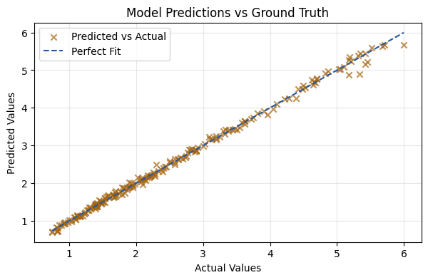
Indeed, the model is trained as it should. The final step is to evaluate its performance on the test set.

y_pred = model(X_test)
mse = mean_squared_error(y_test, y_pred)

print(f"The MSE of the fit is {mse:.5f}")

The MSE of the fit is 0.00562

plt.figure(figsize=(7, 4))
plt.scatter(y_test, y_pred, alpha=0.7, color='#a3630f', marker='x', label='Predicted vs Actual')
plt.plot([y_test.min(), y_test.max()], [y_test.min(), y_test.max()], color='#25599c', linestyle='--', label='Perfect Fit')
plt.xlabel('Actual Values')
plt.ylabel('Predicted Values')
plt.title('Model Predictions vs Ground Truth')
plt.legend()
plt.grid(alpha=0.3)
plt.show()