Tutorial 3 - Initialization Types

Having worked with different layer types, for this tutorial we will stick to Chebyshev-based KANs in order to explore different initialization strategies. Once again, we will be re-using the code shown in the previous notebooks for the definition, training and evaluation of the models.

from jaxkan.models.KAN import KAN

import jax
import jax.numpy as jnp

from sklearn.model_selection import train_test_split
from sklearn.metrics import mean_squared_error

from flax import nnx
import optax

import matplotlib.pyplot as plt
import numpy as np

import os
os.environ["TF_CPP_MIN_LOG_LEVEL"] = "2"

Experiment Setup

def f(x,y):
    return x**2 + 2*jnp.exp(y)

def generate_data(minval=-1, maxval=1, num_samples=1000, seed=42):
    key = jax.random.PRNGKey(seed)
    x_key, y_key = jax.random.split(key)

    x1 = jax.random.uniform(x_key, shape=(num_samples,), minval=minval, maxval=maxval)
    x2 = jax.random.uniform(y_key, shape=(num_samples,), minval=minval, maxval=maxval)

    y = f(x1, x2).reshape(-1, 1)
    X = jnp.stack([x1, x2], axis=1)

    return X, y

seed = 42

X, y = generate_data(minval=-1, maxval=1, num_samples=1000, seed=seed)

X_train, X_test, y_train, y_test = train_test_split(X, y, test_size=0.2, random_state=seed)

print("Training set size:", X_train.shape)
print("Test set size:", X_test.shape)

# Define the static parameters
n_in = X_train.shape[1]
n_out = y_train.shape[1]
n_hidden = 6

layer_dims = [n_in, n_hidden, n_hidden, n_out]

Training set size: (800, 2)
Test set size: (200, 2)

As in the previous notebook, we define a function that incorporates everything. Here, we set init_scheme as its only input, in order to investigate different initialization strategies.

def run_experiment(init_scheme):

    layer_type = "chebyshev"

    required_parameters = {'D': 5, 'flavor': 'exact',
                           'residual': None, 'external_weights': False,
                           'init_scheme': init_scheme,
                           'add_bias': True}

    # Initialize a KAN model, depending on the inputs of the experiment
    model = KAN(layer_dims = layer_dims,
                layer_type = layer_type,
                required_parameters = required_parameters,
                seed = 42
               )

    # Define Optimizer
    opt_type = optax.adam(learning_rate=0.001)
    optimizer = nnx.Optimizer(model, opt_type, wrt=nnx.Param)

    # Define train loop
    @nnx.jit
    def train_step(model, optimizer, X_train, y_train):

        def loss_fn(model):
            residual = model(X_train) - y_train
            loss = jnp.mean((residual)**2)

            return loss

        loss, grads = nnx.value_and_grad(loss_fn)(model)
        optimizer.update(model, grads)

        return loss

    # Do training
    num_epochs = 2000
    train_losses = jnp.zeros((num_epochs,))

    for epoch in range(num_epochs):
        # Calculate the loss
        loss = train_step(model, optimizer, X_train, y_train)

        # Append the loss
        train_losses = train_losses.at[epoch].set(loss)

    # Get MSE on test set
    y_pred = model(X_test)
    mse = mean_squared_error(y_test, y_pred)

    print(f"The MSE of the fit is {mse:.5f}\n\n")

    # Plot Losses
    plt.figure(figsize=(7, 4))

    plt.plot(np.array(train_losses), label='Train Loss', marker='o', color='#25599c', markersize=1)

    plt.xlabel('Epochs')
    plt.ylabel('Loss')
    plt.title('Training Loss Over Epochs')
    plt.yscale('log')

    plt.legend()
    plt.grid(True, which='both', linestyle='--', linewidth=0.5)

    plt.show()

    return

Experiments

We will then run this function with different initialization techniques.

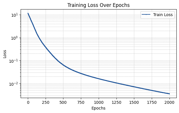
Default Initialization

The default initialization corresponds to the first initialization type introduced for each KAN layer in the paper that proposed it.

init_scheme = {"type": "default"}

run_experiment(init_scheme)

The MSE of the fit is 0.00563

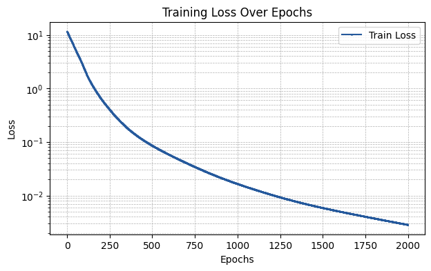
LeCun Initialization

The lecun initialization corresponds to the LeCun-inspired initialization introduced in Initialization Schemes for Kolmogorov–Arnold Networks: An Empirical Study. See the paper for more details.

Note that this initialization includes additional parameters for the init_scheme dictionary.

• distribution: Corresponds to the distribution used to create a sample from which to draw all expectation values involved in the initialization process.

• sample_size: Defines the size of the aforementioned sample.

• gain: Introduces a multiplicative factor for the standard distribution of the initialized weights.

init_scheme = {"type": "lecun", "distribution": "uniform", "sample_size": 10000, "gain": None}

run_experiment(init_scheme)

The MSE of the fit is 0.00630

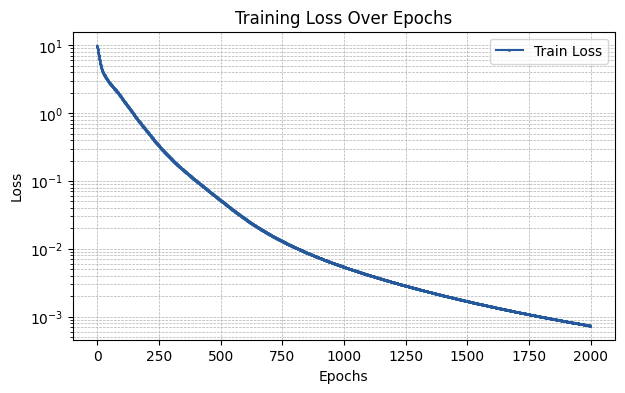
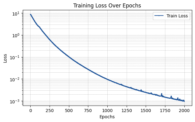
Glorot Initialization

The glorot initialization corresponds to the Glorot-inspired initialization introduced in Initialization Schemes for Kolmogorov–Arnold Networks: An Empirical Study. See the paper for more details.

init_scheme = {"type": "glorot", "distribution": "uniform", "sample_size": 10000, "gain": None}

run_experiment(init_scheme)

The MSE of the fit is 0.00090

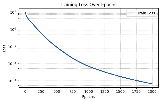
Fine Glorot Initialization

The glorot_fine initialization corresponds to the Glorot-inspired initialization introduced in Training Deep Physics-Informed Kolmogorov-Arnold Networks. Essentially, it’s a basis-function-term-dependent initialization, which introduces a different standard deviation per basis function term. See the paper for more details.

init_scheme = {"type": "glorot_fine", "distribution": "uniform", "sample_size": 10000, "gain": None}

run_experiment(init_scheme)

The MSE of the fit is 0.00090

Power-Law Initialization

The power initialization corresponds to a generalization of the power-law initialization introduced in Initialization Schemes for Kolmogorov–Arnold Networks: An Empirical Study.

In its more general form, this initialization initializes residual and basis weights following \(\mathcal{N}\left(0, \sigma_r^2\right)\) and \(\mathcal{N}\left(0, \sigma_b^2\right)\), respectively, where

\[\sigma_r = c_r \times \frac{1}{n_\text{in}^{\alpha_1} \times \left(D+1\right)^{\alpha_2}} \qquad \sigma_b = c_b \times \frac{1}{n_\text{in}^{\beta_1} \times \left(D+1\right)^{\beta_2}},\]

with \(D\) being equal to \(G+k\) for spline-based KAN layers.

See the paper for more details, where \(c_r = c_b = 1.0\), \(\alpha_1 = \alpha_2 = \alpha\) and \(\beta_1 = \beta_2 = \beta\).

init_scheme = {"type": "power", "const_b": 1.0, "const_r": 1.0, "pow_b1": 1.75, "pow_b2": 1.75, "pow_r1": 0.25, "pow_r2": 0.25}

run_experiment(init_scheme)

The MSE of the fit is 0.00127