Tutorial 10 - Advanced Models for PDEs

In this tutorial we will be addressing a forward PDE problem using an architecture more advanced than the standard KAN used in Tutorial 8.

from jaxkan.models.RGAKAN import RGAKAN

import jax
import jax.numpy as jnp

from jaxkan.pikan.pde import get_ac_res
from jaxkan.pikan.sampling import get_collocs_grid
from jaxkan.pikan.adaptive import (
    apply_rba_weights,
    get_causal_weights,
    get_colloc_indices,
    get_rad_indices,
    lr_anneal,
    update_rba_weights,
)

from typing import Union, List

from flax import nnx
import optax

import matplotlib.pyplot as plt
import numpy as np

import os
os.environ["TF_CPP_MIN_LOG_LEVEL"] = "3"

Data Generation

We will once again be solving the Allen-Cahn Equation,

\[\frac{\partial u}{\partial t} - D\frac{\partial^2 u}{\partial x^2} + 5 \left(u^3 - u\right) = 0,\]

for \(D = 10^{-4}\) in the \(\Omega = [0,1]\times [-1, 1]\) domain, subject to initial condition

\[u\left(t=0, x\right) = x^2 \cos\left(\pi x\right),\]

and periodic boundary conditions

\[u\left(t, x=-1\right) = u\left(t, x=1\right).\]

Again, we will be using adaptive training methods (see Tutorial 8 and this paper).

seed = 42

# Generate Collocation points for PDE
collocs_pool = get_collocs_grid(ranges=[(0, 1, 2**7), (-1, 1, 2**7)])

# Generate Collocation points for IC
ic_collocs = get_collocs_grid(ranges=[(0, 0, 1), (-1, 1, 2**6)])
ic_data = ((ic_collocs[:,1]**2)*jnp.cos(jnp.pi*ic_collocs[:,1])).reshape(-1,1)

RGA KAN Model

Instead of using the vanilla KAN model, we will be using the Residual-Gated Adaptive Kolmogorv-Arnold Network introduced in Training Deep Physics-Informed Kolmogorov-Arnold Networks. Once again, boundary conditions will be enforced directly via the model architecture, this time by applying periodical embeddings (see the API Reference of RGAKAN).

# Initialize an RGA KAN model
n_in = collocs_pool.shape[1]
n_out = 1
n_hidden = 8
num_blocks = 2
flavor = 'exact'
D = 5
init_scheme = {'type': 'glorot_fine'}
alpha = 0.0
beta = 0.0
ref = None
period_axes = {1 : (jnp.pi, False)}
rff_std = None
sine_D = 5

model = RGAKAN(n_in = n_in, n_out = n_out, n_hidden = n_hidden, num_blocks = num_blocks, flavor = flavor, D = D,
               init_scheme = init_scheme, alpha = alpha, beta = beta, ref = ref, period_axes = period_axes,
               rff_std = rff_std, sine_D = sine_D, seed = seed)

# We will also be using a more adaptive optimizer with learning rate scheduling
lr_schedule = optax.exponential_decay(
                init_value=1e-3,
                transition_steps=1000,
                decay_rate=0.9,
                staircase=False
            )

opt_type = optax.adam(learning_rate=lr_schedule, b1=0.9, b2=0.999, eps=1e-8)

optimizer = nnx.Optimizer(model, opt_type, wrt=nnx.Param)

Adaptive Training

@nnx.jit
def get_rad_collocs(model, pde_collocs_pool, sorted_indices, l_pde, l_pde_pool):
    resids_pool = pde_res(model, pde_collocs_pool)
    new_indices, new_pool, _ = get_rad_indices(
        collocs_pool=pde_collocs_pool,
        residuals=resids_pool,
        old_indices=sorted_indices,
        batch_weights=l_pde,
        pool_weights=l_pde_pool,
        batch_size=batch_size,
        rad_a=rad_a,
        rad_c=rad_c,
        seed=seed,
    )
    return new_indices, new_pool

# PDE Residual
pde_res = get_ac_res()

# PDE Loss
def pde_loss(model, l_E, collocs):

    residuals = pde_res(model, collocs) # shape (batch_size, 1)

    # Get new RBA weights
    l_E_new = update_rba_weights(residuals, l_E, gamma=RBA_gamma, eta=RBA_eta)

    # Multiply by RBA weights while keeping them out of the backward graph
    w_resids = apply_rba_weights(residuals, l_E_new)

    # Reshape residuals for causal training
    residuals = w_resids.reshape(num_chunks, -1) # shape (num_chunks, points)

    # Get average loss per chunk
    loss = jnp.mean(residuals**2, axis=1)

    # Get causal weights
    weights = get_causal_weights(loss, M, causal_tol)

    # Weighted loss
    weighted_loss = jnp.mean(weights * loss)

    return weighted_loss, l_E_new


def ic_loss(model, l_I, ic_collocs, ic_data):

    # Residual
    ic_res = model(ic_collocs) - ic_data

    # Get new RBA weights
    l_I_new = update_rba_weights(ic_res, l_I, gamma=RBA_gamma, eta=RBA_eta)

    # Multiply by RBA weights while keeping them out of the backward graph
    w_resids = apply_rba_weights(ic_res, l_I_new)

    # Loss
    loss = jnp.mean(w_resids**2)

    return loss, l_I_new


@nnx.jit(static_argnames=("compute_grads_sep",))
def train_step(model, optimizer, collocs, ic_collocs, ic_data, λ_E, λ_I, l_E, l_I, compute_grads_sep=False):

    def total_loss_fn(model):
        (loss_E, l_E_new) = pde_loss(model, l_E, collocs)
        (loss_I, l_I_new) = ic_loss(model, l_I, ic_collocs, ic_data)
        total = λ_E * loss_E + λ_I * loss_I
        return total, (loss_E, loss_I, l_E_new, l_I_new)

    (loss, aux), grads = nnx.value_and_grad(total_loss_fn, has_aux=True)(model)

    sep_grads = (None, None)
    if compute_grads_sep:
        grads_E = nnx.grad(lambda m: pde_loss(m, l_E, collocs)[0])(model)
        grads_I = nnx.grad(lambda m: ic_loss(m, l_I, ic_collocs, ic_data)[0])(model)
        sep_grads = (grads_E, grads_I)

    optimizer.update(model, grads)

    return loss, aux, sep_grads

num_epochs = 10_000

# Define causal training parameters
causal_tol = 1.0
num_chunks = 32
M = jnp.triu(jnp.ones((num_chunks, num_chunks)), k=1).T

# Define LR Annealing parameters
grad_mixing = 0.9
f_grad_norm = 1000

# Define resampling parameters
batch_size = 2**12
f_resample = 2000
rad_a = 1.0
rad_c = 1.0

# Define RBA parameters
RBA_gamma = 0.999
RBA_eta = 0.01

# Initialize RBA weights - full pool
l_E_pool = jnp.ones((collocs_pool.shape[0], 1))
# Also get RBAs for ICs
l_I = jnp.ones((ic_collocs.shape[0], 1))

# Get starting collocation points & RBA weights
sorted_indices = get_colloc_indices(collocs_pool=collocs_pool, batch_size=batch_size, px=None, seed=seed)

pde_collocs = collocs_pool[sorted_indices]
l_E = l_E_pool[sorted_indices]

# Define global loss weights (initialization)
λ_E = jnp.array(1.0, dtype=float)
λ_I = jnp.array(1.0, dtype=float)

Following this setup, we proceed to train the model.

train_losses = jnp.zeros((num_epochs,))

# Start training
for epoch in range(num_epochs):

    do_anneal = (epoch != 0) and (epoch % f_grad_norm == 0)

    loss, aux, sep_grads = train_step(
        model, optimizer, pde_collocs, ic_collocs, ic_data, λ_E, λ_I, l_E, l_I,
        compute_grads_sep=do_anneal
    )

    loss_E, loss_I, l_E, l_I = aux

    # Perform lr annealing
    if do_anneal:

        print(f"Epoch No. {epoch}. Current loss: {loss:.2e}. Performing learning-rate annealing.")

        λ_E, λ_I = lr_anneal((sep_grads[0], sep_grads[1]), (λ_E, λ_I), grad_mixing)

    # Perform RAD
    if (epoch != 0) and (epoch % f_resample == 0):

        print(f"Epoch No. {epoch}. Current loss: {loss:.2e}. Performing RAD resampling.")

        sorted_indices, l_E_pool = get_rad_collocs(
            model, collocs_pool, sorted_indices, l_E, l_E_pool
        )

        # Set new batch of collocs and l_E
        pde_collocs = collocs_pool[sorted_indices]
        l_E = l_E_pool[sorted_indices]

    # Append the loss
    train_losses = train_losses.at[epoch].set(loss)

Epoch No. 1000. Current loss: 1.46e-02. Performing learning-rate annealing.
Epoch No. 2000. Current loss: 3.24e-02. Performing learning-rate annealing.
Epoch No. 2000. Current loss: 3.24e-02. Performing RAD resampling.
Epoch No. 3000. Current loss: 4.50e-02. Performing learning-rate annealing.
Epoch No. 4000. Current loss: 1.05e-03. Performing learning-rate annealing.
Epoch No. 4000. Current loss: 1.05e-03. Performing RAD resampling.
Epoch No. 5000. Current loss: 8.24e-04. Performing learning-rate annealing.
Epoch No. 6000. Current loss: 7.38e-04. Performing learning-rate annealing.
Epoch No. 6000. Current loss: 7.38e-04. Performing RAD resampling.
Epoch No. 7000. Current loss: 5.36e-04. Performing learning-rate annealing.
Epoch No. 8000. Current loss: 6.69e-04. Performing learning-rate annealing.
Epoch No. 8000. Current loss: 6.69e-04. Performing RAD resampling.
Epoch No. 9000. Current loss: 5.53e-04. Performing learning-rate annealing.

Evaluation

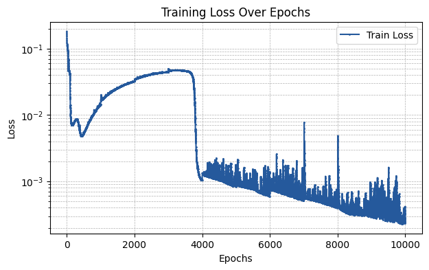
By visualizing the train loss curve, we can see that even when training for a significantly smaller number of epochs than in the vanilla KAN case, the loss function decreases further.

plt.figure(figsize=(7, 4))

plt.plot(np.array(train_losses), label='Train Loss', marker='o', color='#25599c', markersize=1)

plt.xlabel('Epochs')
plt.ylabel('Loss')
plt.title('Training Loss Over Epochs')
plt.yscale('log')

plt.legend()
plt.grid(True, which='both', linestyle='--', linewidth=0.5)

plt.show()

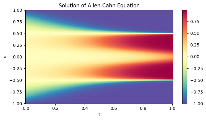
Additionally, the approximation to the actual solution is better.

N_t, N_x = 100, 256

t = np.linspace(0.0, 1.0, N_t)
x = np.linspace(-1.0, 1.0, N_x)
T, X = np.meshgrid(t, x, indexing='ij')
coords = np.stack([T.flatten(), X.flatten()], axis=1)

output = model(jnp.array(coords))
resplot = np.array(output).reshape(N_t, N_x)

plt.figure(figsize=(7, 4))
plt.pcolormesh(T, X, resplot, shading='auto', cmap='Spectral_r')
plt.colorbar()

plt.title('Solution of Allen-Cahn Equation')
plt.xlabel('t')

plt.ylabel('x')

plt.tight_layout()
plt.show()