Tutorial 9 - Inverse PDE Problem

In this tutorial we will be working with the DIY KAN concept once again, this time in order to solve an inverse PDE problem.

from typing import List
from jaxkan.layers.Spline import SplineLayer

import jax
import jax.numpy as jnp

from jaxkan.pikan.sampling import get_collocs_sobol

from flax import nnx
import optax

import matplotlib.pyplot as plt
import numpy as np

import os
os.environ["TF_CPP_MIN_LOG_LEVEL"] = "3"

Data Generation

For the purposes of this example, we will be working with the Diffusion Equation,

\[\frac{\partial u}{\partial t} -D \frac{\partial^2 u}{\partial x^2} = 0,\]

in the \(\Omega = [0,1]\times [0,1]\) domain, subject to the boundary conditions

\[u\left(t=0, x\right) = \sin\left(\pi x\right),\]

\[u\left(t, x=0\right) = u\left(t, x=1\right) = 0.\]

We have intentionally left \(D\) undefined, as we intend to also estimate it (apart from solving the PDE), using “experimental data”. The PDE’s analytical solution is given by

\[u(t,x) = \sin\left(\pi x\right) \cdot \exp\left(-D\pi^2 t\right),\]

so it will be used to generate mock experimental data with gaussian noise for \(D = 0.25\).

seed = 42

# Generate Collocation points for PDE
pde_collocs = get_collocs_sobol(ranges=[(0,1), (0,1)], total_points=2**12, seed=seed)

# Generate Collocation points for IC
ic_collocs = get_collocs_sobol(ranges=[(0,0), (0,1)], total_points=2**6, seed=seed)
ic_data = jnp.sin(np.pi*ic_collocs[:,1]).reshape(-1,1)

# Generate Collocation points for BCs
bc1_collocs = get_collocs_sobol(ranges=[(0,1), (0,0)], total_points=2**6, seed=seed)
bc1_data = jnp.zeros(bc1_collocs.shape[0]).reshape(-1,1)

bc2_collocs = get_collocs_sobol(ranges=[(0,1), (1,1)], total_points=2**6, seed=seed)
bc2_data = jnp.zeros(bc2_collocs.shape[0]).reshape(-1,1)

# Concatenate IC/BCs
bc_collocs = jnp.concatenate([ic_collocs, bc1_collocs, bc2_collocs], axis=0)
bc_data = jnp.concatenate([ic_data, bc1_data, bc2_data], axis=0)

# Generate experimental data for inverse problem
def u(t, x, tau):
    return jnp.sin(jnp.pi*x)*jnp.exp(-tau*(jnp.pi**2)*t)

key = jax.random.PRNGKey(seed)
idxs = jax.random.choice(key, jnp.arange(pde_collocs.shape[0]), (1000,), replace=False)
exp_collocs = pde_collocs[idxs]

u_vals = u(exp_collocs[:,0], exp_collocs[:,1], 0.25).reshape(-1,1)
noise = u_vals.std()*jax.random.normal(key, shape=(1000,1))
exp_data = u_vals + noise

KAN Model

We will define a KAN Class based on the Spline Layer, which will also include a trainable parameter, \(\tau\).

class MyKAN(nnx.Module):

    def __init__(self, layer_dims: List[int], k: int = 3, G: int = 5, add_bias: bool = True, seed: int = 42):

        self.layers = nnx.List([
                SplineLayer(
                    n_in=layer_dims[i],
                    n_out=layer_dims[i + 1],
                    k=k,
                    G=G,
                    residual=nnx.silu,
                    external_weights=True,
                    add_bias=add_bias,
                    seed=seed)
                for i in range(len(layer_dims) - 1)
            ])

        # This is the parameter we need to identify to solve the inverse problem
        # We initialize it at 1.0
        self.tau = nnx.Param(jnp.array([1.0]))


    def __call__(self, x):

        for layer in self.layers:
            x = layer(x)

        return x

# Initialize a MyKAN model instance
n_in = pde_collocs.shape[1]
n_out = 1
n_hidden = 6

layer_dims = [n_in, n_hidden, n_hidden, n_out]

model = MyKAN(layer_dims = layer_dims, k = 3, G = 5, add_bias = True, seed = 42)

Training

PIKANs provide a unified framework for solving the forward and the inverse PDE problem. Nonetheless, we will need to incorporate the “experimental” data in the loss function.

opt_type = optax.adam(learning_rate=0.001)

optimizer = nnx.Optimizer(model, opt_type, wrt=nnx.Param)

# PDE Loss
def pde_loss(model, collocs):
    tau = model.tau[0]

    def u_fn(t, x):
        return model(jnp.array([[t, x]]))[0, 0]

    u_t_fn = jax.grad(u_fn, argnums=0)
    u_x_fn = jax.grad(u_fn, argnums=1)
    u_xx_fn = jax.grad(u_x_fn, argnums=1)

    pde_res = jax.vmap(
        lambda t, x: u_t_fn(t, x) - tau * u_xx_fn(t, x),
        in_axes=(0, 0),
    )(collocs[:, 0], collocs[:, 1]).reshape(-1, 1)

    return pde_res

# Define train loop
@nnx.jit
def train_step(model, optimizer, collocs, bc_collocs, bc_data, exp_collocs, exp_data):

    def loss_fn(model):
        # PDE part
        pde_res = pde_loss(model, collocs)
        total_loss = jnp.mean((pde_res)**2)

        # IC/BC part
        bc_res = model(bc_collocs) - bc_data
        total_loss += jnp.mean(bc_res**2)

        # Experimental data loss
        exp_res = model(exp_collocs) - exp_data
        total_loss += jnp.mean(exp_res**2)

        return total_loss

    loss, grads = nnx.value_and_grad(loss_fn)(model)
    optimizer.update(model, grads)

    return loss

# Initialize train_losses
num_epochs = 5000

for epoch in range(num_epochs):
    # Calculate the loss
    loss = train_step(model, optimizer, pde_collocs, bc_collocs, bc_data, exp_collocs, exp_data)

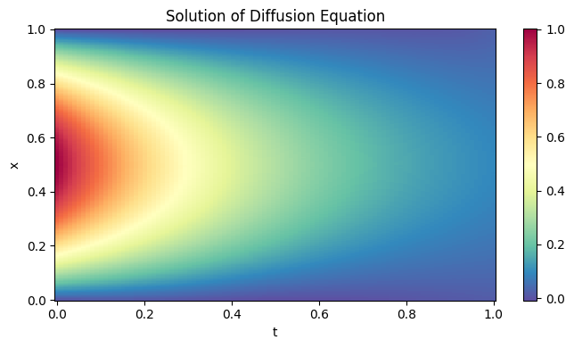
Evaluation

The following plot shows the trained neural network on the entire domain, approximating the solution, \(u\), of the equation.

N_t, N_x = 100, 256

t = np.linspace(0.0, 1.0, N_t)
x = np.linspace(0.0, 1.0, N_x)
T, X = np.meshgrid(t, x, indexing='ij')
coords = np.stack([T.flatten(), X.flatten()], axis=1)

output = model(jnp.array(coords))
resplot = np.array(output).reshape(N_t, N_x)

plt.figure(figsize=(7, 4))
plt.pcolormesh(T, X, resplot, shading='auto', cmap='Spectral_r')
plt.colorbar()

plt.title('Solution of Diffusion Equation')
plt.xlabel('t')

plt.ylabel('x')

plt.tight_layout()
plt.show()

We can also visualize the difference between the analytical and the approximated solution.

output = model(jnp.array(coords))
diff = output - u(coords[:,0], coords[:,1], 0.25).reshape(-1, 1)
resplot = np.array(diff).reshape(N_t, N_x)

plt.figure(figsize=(7, 4))
plt.pcolormesh(T, X, resplot, shading='auto', cmap='Spectral_r')
plt.colorbar()

plt.title('Difference between approximated and analytical solution')
plt.xlabel('t')

plt.ylabel('x')

plt.tight_layout()
plt.show()

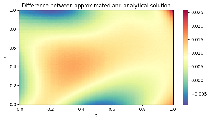
It appears that the approximation is good, since the maximum absolute error is \(\sim 0.02\).

Finally, we can see that \(\tau\) is approximated quite well:

print(f"The approximated value for τ is {model.tau[0]}.")

The approximated value for τ is 0.24094036221504211.